↜ Back to index Introduction to Numerical Analysis 1

Today we talk more about the numerical scheme for the heat equation that we derived in Lecture b1.

Numerical scheme for the heat equation in Fortran

Here is an example Fortran code for the case a = b = 0 and u_0(x) = \sin(\pi x), M = 10 and \tau = h^2 / 4. The exact solution is expected to be u(x,t) = \exp(-\pi^2 t) \sin(\pi x).

implicit none
! introduce constants M and pi
integer, parameter :: M = 10
real, parameter :: pi = 4. * atan(1.)
integer n, k, nmax
real h, tau, x
! We use arrays to store the values of u_n (in u) and u_{n+1} (in v)
!                  The arrays will be indexed from 0 to M.
!               👇 M must be a constant to be used here.
real, dimension(0:M) :: u, v

h = 1. / M
tau = h * h / 4.
!      👇 we solve the problem up to time t_nmax = 0.5
nmax = 0.5 / tau

! Initialize u with the initial data u_0 and print the values.
! Since sin(0) = sin(pi) = 0 = a = b, we do not need to set the boundary data
! separately.
do k=0, M
    x = k * h
    u(k) = sin(pi * x)
end do
! Print the initial data
 call printstep(0., u)

do n=0, nmax-1
    ! One step of the finite difference method from u_n to u_{n+1}
    ! Array u holds the values of u_n.
    ! Array v will be filled with computed values of u_{n+1}.

    v(0) = u(0) ! boundary condition is constant in time
    do k = 1, M-1
        v(k) = u(k) + (tau / (h * h)) * (u(k - 1) - 2 * u(k) + u(k + 1))
    end do
    v(M) = u(M) ! boundary condition is constant in time

    ! Print the solution
    call printstep((n+1) * tau, v)

    ! store the values of v in u
    u = v
end do
 contains
    ! Prints the values of the solution at a given time step
    subroutine printstep(tn, un)
        real tn
        real, dimension(0:M) :: un
        integer k
        do k = 0, M
            print *, tn, k * h, un(k)
        end do
        ! print an empty line (needed for gnuplot)
        print *
    end subroutine
end

The output consists of values t_n, x_k and u_{n, k}, one (n, k) per line.

   0.00000000       0.00000000       0.00000000    
   0.00000000      0.100000001      0.309017003    
   0.00000000      0.200000003      0.587785244    
   0.00000000      0.300000012      0.809017062    
   0.00000000      0.400000006      0.951056540    
   0.00000000      0.500000000       1.00000000    
   0.00000000      0.600000024      0.951056480    
   0.00000000      0.699999988      0.809017003    
   0.00000000      0.800000012      0.587785184    
   0.00000000      0.900000036      0.309016794    
   0.00000000       1.00000000      -8.74227766E-08

   2.50000018E-03   0.00000000       0.00000000    
   2.50000018E-03  0.100000001      0.301454812    
   2.50000018E-03  0.200000003      0.573401153    
   ...

Plotting the solution

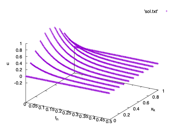
We included an empty line after the data for each time step to allow gnuplot understand that this data is on a regular two dimensional grid. To plot such two dimensional data in gnuplot, we use splot instead of plot.

First we save the output in a file, say sol.txt.

$ ./a.exe > sol.txt

Then in gnuplot we can plot the data using the following commands.

set xlabel 't_n'
set ylabel 'x_k'
set zlabel 'u'
splot 'sol.txt'

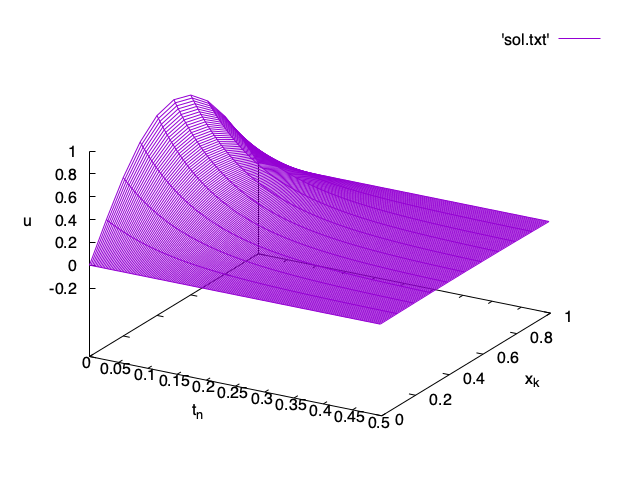
This is a bit difficult to understand, so we usually connect the points of the solution into a mesh that is a bit easier to read, by adding w l to the splot command:

splot 'sol.txt' w l

Here w l is a shorthand for with lines.

Note how much smaller the time step \tau is compared to the space step h. Unfortunately, with the numerical method discussed here we need to choose \tau \leq \frac{h^2}2. We will discuss this in more detail later. Try to change \tau to h^2 in the program and see what happens to the solution.

Making an animation

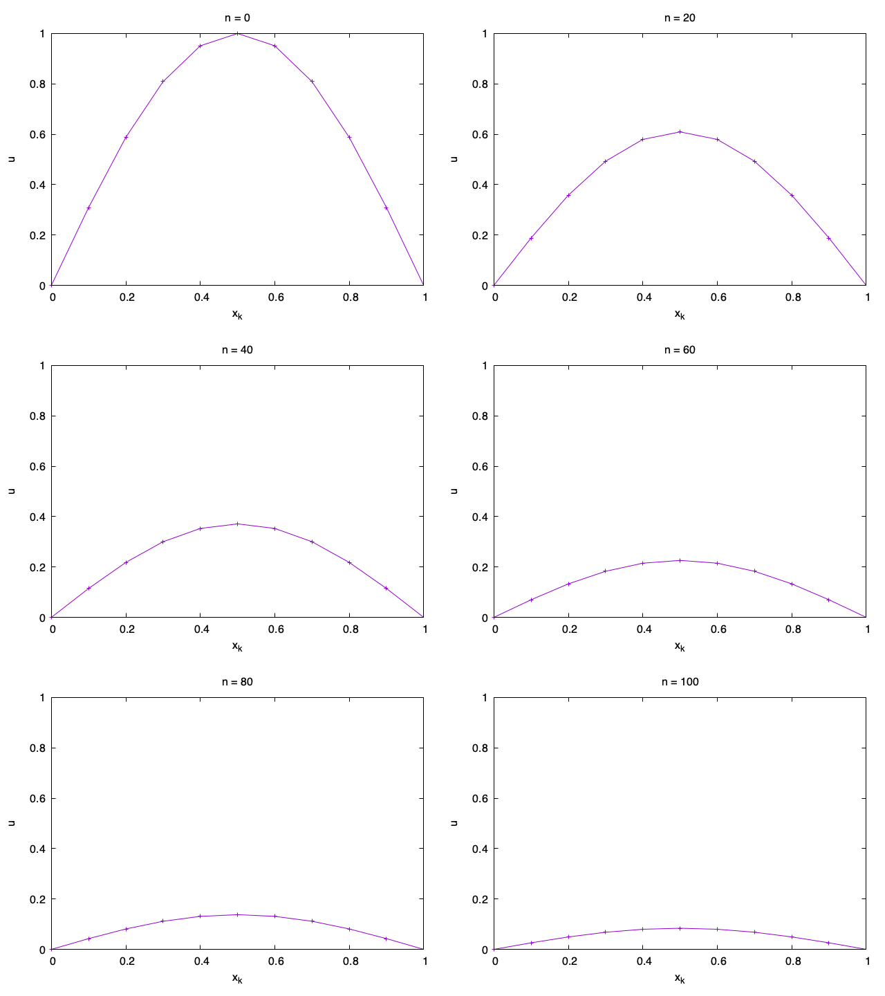
However, since the solution depends on time, it is often best to plot the solution as a sequence of graphs of u_{n, k} as a function of x_k, one for each n.

To plot only the graph for one time step as in the animation above, say n=42, you can use the gnuplot commands

plot 'sol.txt' every :::42::42 using 2:3 w linespoints

The command that selects the 42nd time step is every :::42::42. The number of : characters is important. For more on this syntax see How do I plot a part of data in a file ?.

Plotting using a contour plot

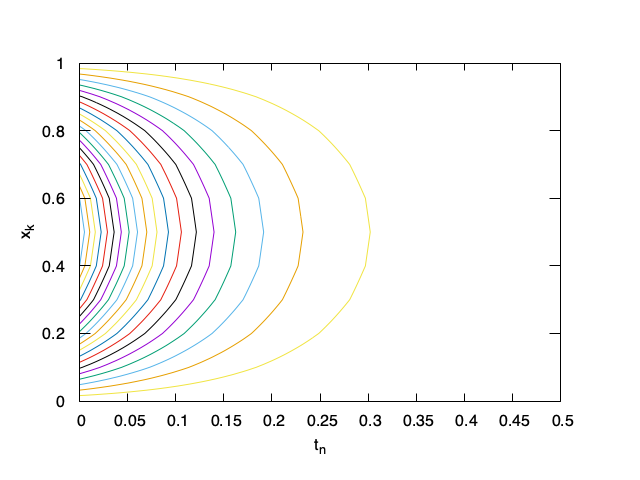
Another useful way of plotting the solution is using a contour plot to plot the curves along which the solution is constant. It is very similar to what we did in Lecture a5.

set view map
unset surface
set contour
set cntrparam levels 30
unset key
set xlabel 't_n'
set ylabel 'x_k'
splot 'sol.txt' w l